Keep the same guitar and the same string, but move your finger a little closer to the bridge: the sound may become brighter. The instrument has not changed, and the pitch is almost the same. Where does the difference begin?To understand guitar acoustics, follow a single pluck and see how it becomes the sound we hear.
Following the video, this article connects plucking, body–air coupling, damping, sound propagation and hearing. Ten interactive models replace repeated explanations, alongside key equations and measurement photographs. The A/B sounds and simulated curves are teaching examples, not recordings or measurements of a real guitar.
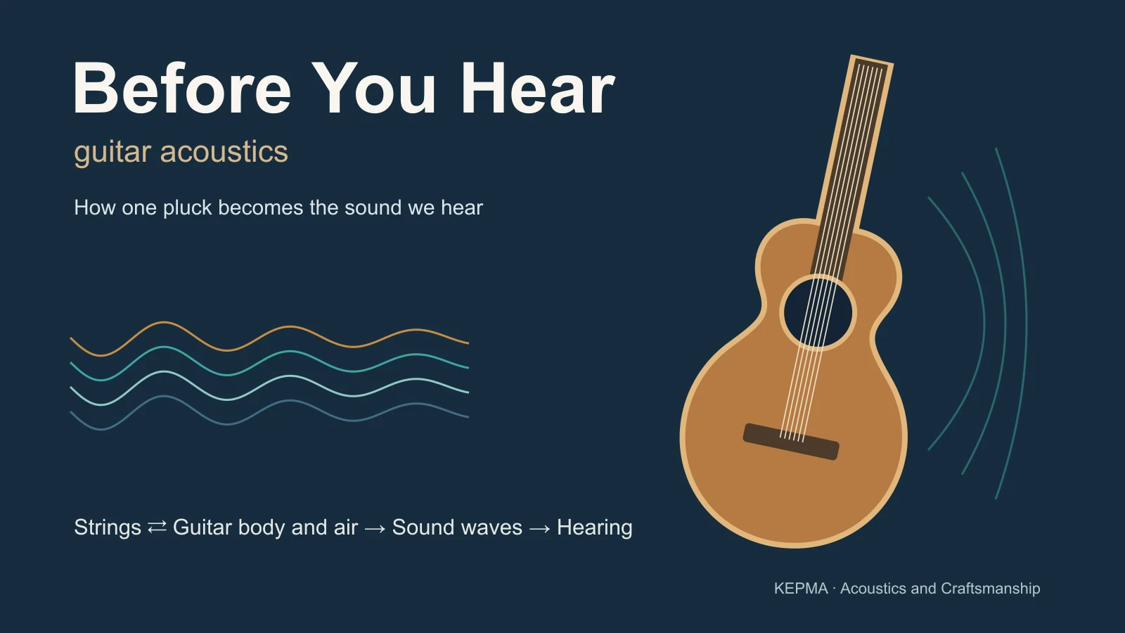 Play the full videoPlay on this page · 08:16 · Bilibili
First, see the whole route
The film begins with acoustic oscillations in the early universe before returning to a string close at hand. Both can be discussed using vibration, modes, and spectra, but their scales, media, and dynamics are different. Those early oscillations occurred in the tightly coupled fluid of matter and radiation that existed at the time. They do not imply that sound can travel through the vacuum of space today.
For a guitar, the process begins with a specific action. A finger pulls the string aside, and the work done by that external force stores mechanical energy in the system. After release, the system moves according to its initial state and dynamics. The string exchanges energy with the body through the bridge. The soundboard, back, and air interact and radiate sound. We need not memorize every term at once. First, identify the question each stage answers.
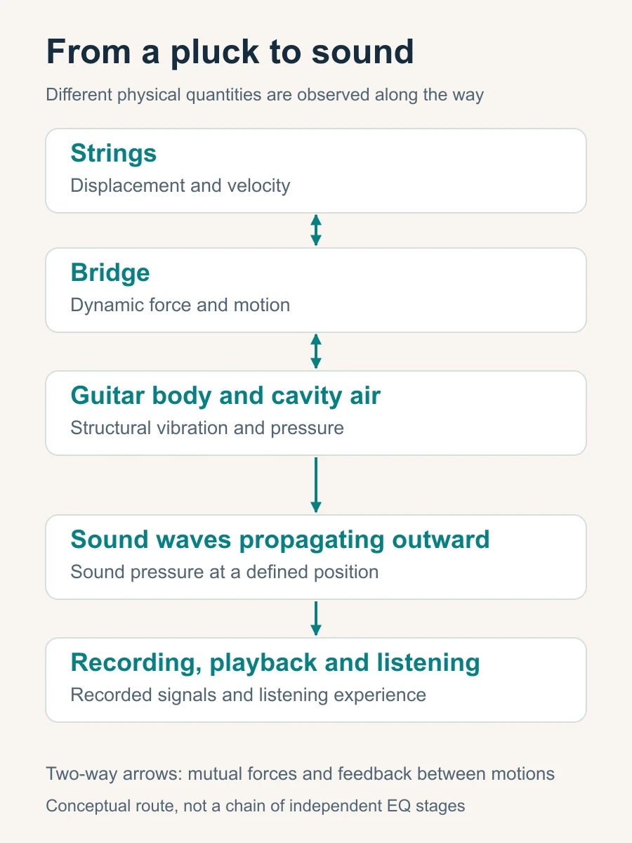
Signals describe how quantities change. Energy tells us how work is done and where it goes. String displacement, the dynamic force at the bridge, and sound pressure in air can all be plotted as signals over time. A waveform alone, however, does not tell us how much energy crosses an interface. Keeping these questions separate helps avoid confusion between spectra, coupling, and damping.
Two inputs with the same fundamental
Adjustable teaching modelTry it · Set both A and B to 0.50 and listen. Then change only one plucking position and compare the waveforms and sound.
1. What the fingers leave behind: more than playing strength
Video reference: approximately 00:39–01:03
From an initial shape to propagation and reflection
When a finger holds a string aside, its shape is already displaced from equilibrium. For the moment, assume an ideal string: uniform, perfectly flexible, under constant tension, and fixed at both ends. If finger contact is reduced to a point, the shape before release is approximately a triangle made from two straight segments. At release, the subsequent motion inherits the initial displacement of the entire string and its initial velocity.
The shape matters. The system does not receive only one number called playing harder. Plucking position, displacement, direction, contact width, and release speed can all change the initial state or release process. Pulling the string slowly and releasing it need not produce the same input as a pick sweeping quickly across it. A slow pull may also cause small, nearly static deformations of the body. A precise prediction must account for those initial states too.
After release, disturbances travel along the string, reflect at the ends, and combine with other travelling components. At an ideal fixed end, displacement must remain zero, so reflection involves the corresponding inversion. The resulting motion can be understood through propagation and reflection or described as a combination of standing waves. These are two views of the same motion.
What determines pitch first?
An ideal string’s fundamental frequency is governed mainly by its vibrating length, tension, and linear density. Linear density means mass per unit length, rather than the name of a material. With other conditions unchanged, a shorter string or higher tension raises the fundamental. Greater linear density lowers it. Familiar actions such as fretting to shorten the string and tuning to change its tension follow directly from this relationship.
f₁ ≈ (1 / 2L) √(T / μ)
Here f₁ is the ideal string’s fundamental frequency, L its vibrating length, T its tension, and μ its linear density. This is an introductory relationship. Real-string stiffness, winding construction, and flexible terminations require corrections.
The film uses a vibration near 110 Hz as an example: about 110 cycles per second, or roughly 9 milliseconds per cycle. This describes the rate of string vibration. The speed of transverse waves along the string is a different quantity from the speed of sound in air. Pitch tells us something important about how fast the motion repeats, but not yet why a sound is bright, rounded, or has a particular attack.
The same displacement need not supply the same energy
One detail is easy to miss. Pulling the string aside by the same amount at different positions can still produce different slopes and stored energies. In an ideal example with a length of 0.65 m, tension of 70 N, and displacement of 2 mm, release at one-quarter of the string length stores about 1.15 mJ in the string. Release at the midpoint stores about 0.86 mJ. These are model calculations, not measurements of a particular guitar.
So saying that two plucks have exactly the same strength requires us to specify what was controlled: the hand movement, displacement, pulling force, or actual input energy. Everyday playing need not become a laboratory exercise. For a rigorous timbre comparison, however, keep the action as consistent as possible and repeat it. Next, consider how plucking position changes the proportions of frequency components.
2. One pitch, different timbres
Video reference: approximately 01:00–01:33
Harmonics are components that build the string’s shape
A string note near 110 Hz is usually more than a single 110 Hz sine wave. An ideal string also allows components near 220, 330, 440 Hz, and other integer multiples. Their amplitudes, phases, and changes over time combine to form the complex waveform we observe. The body does not receive a pure low tone and then create every higher component from nothing. Many higher harmonics already exist in the initial string motion.
Arranging components by frequency and strength gives the familiar amplitude spectrum—something like a list of ingredients. Similar fundamentals can accompany different harmonic proportions and therefore different perceived timbres. Phase records where each component is in its cycle and affects how the components combine into a transient waveform. Amplitude without phase cannot uniquely reconstruct the original time signal.
In guitar acoustics, distinguish string modes from body modes as well. The ideal string’s frequency components relate to its standing-wave patterns. The soundboard and complete structure have their own natural patterns, which need not coincide with the string’s integer harmonics. A strong harmonic and an identified body mode are different findings requiring different evidence.
Plucking position changes the recipe first
Near the bridge, the initial shape is sharper and less symmetric. Higher harmonics are generally richer relative to the fundamental, often giving a brighter sound. A midpoint pluck has a particular symmetry. In the ideal model, the midpoint is a node of the even-numbered mode shapes, so that symmetric initial displacement does not excite those terms.
This relationship has conditions. A fingertip, nail, or pick has a finite contact width and release time. The string has stiffness, and the bridge moves. A real spectrum therefore need not contain the perfectly clean zeros of the mathematical model. Changing from finger flesh to nail, or changing the pick angle, may also alter contact, release, and attack noise. Plucking position alone cannot explain every change.
From initial shape to bridge force
Adjustable teaching modelTry it · Set b to 0.50 and inspect the even harmonics. Switch between displacement and bridge force to compare their high-frequency roll-off.
A spectrum also needs a time reference
The spectrum at onset may differ from the spectrum half a second later or during the final decay. The analysis window also affects frequency resolution and the appearance of transients. Averaging the whole note can merge a sharp attack with a rounder decay. That hides how the sound develops.
Use the amplitude spectrum, time envelope and spectrogram together. A spectrum compares components. An envelope shows the rise and fall. Spectrograms track frequency bands over time. Each is a different view. A string-displacement spectrum, a bridge-force spectrum and a microphone-pressure spectrum describe different quantities. Converting string motion into bridge force also involves the string slope at the end.
Reading a spectral display: frequency, time and scale
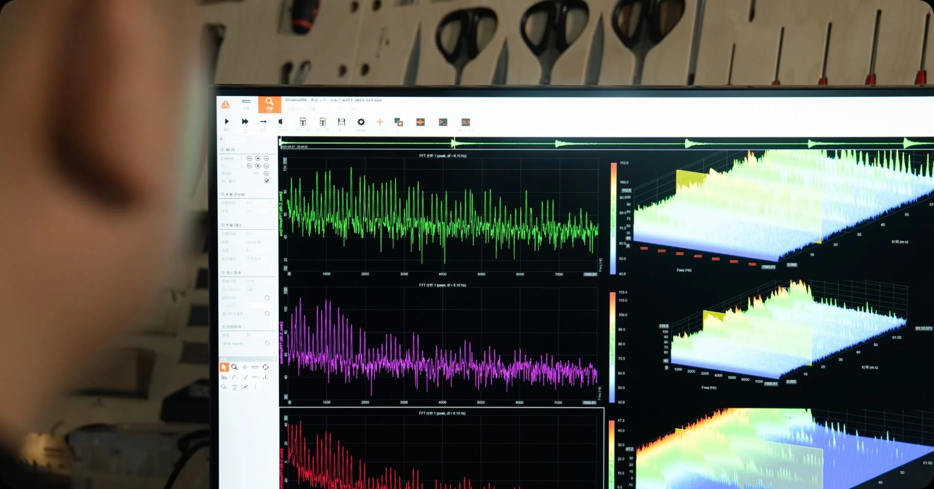
Software estimates a spectrum from a finite signal segment. In the script’s example, 8192 samples at 48 kHz span about 171 milliseconds. The frequency-grid spacing is about 5.86 Hz. This spacing does not guarantee that two peaks 5.86 Hz apart will be resolved. The window function, noise and peak widths also matter.
3. How the bridge connects string motion to the body
Video reference: approximately 01:34–01:43. The coupling section returns to this interface.
Force alone does not establish energy transfer
A thin string can move quickly, yet it radiates sound into the air relatively inefficiently on its own. The bridge transfers the string’s dynamic forces to a larger structure. Motion of the soundboard and other parts then interacts with the air. During ordinary playing, the body has no independent, continuous energy supply. It shapes how the available energy is stored, transferred, dissipated and radiated.
At the bridge, force alone does not determine energy transfer. We also need the velocity of its point of application. Instantaneous power in one direction is force times velocity at the same point, in that direction. Matching signs send energy into the selected body subsystem. Opposite signs can return energy temporarily. Integrating power over a stated time interval gives the net energy transferred.
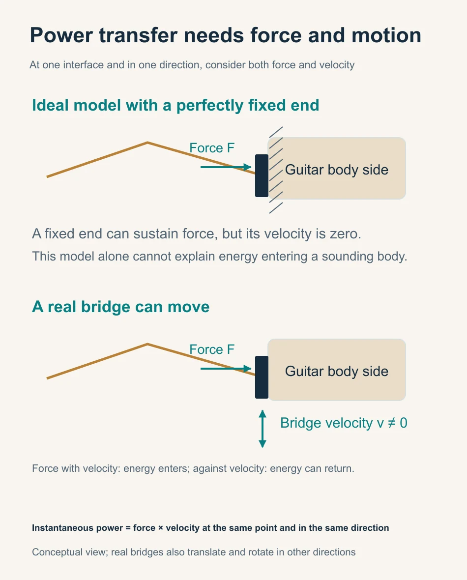
This marks a limit of the fixed-end string model. Perfectly fixed endpoints help explain standing waves and excitation spectra. They cannot also predict exactly how much energy enters a moving, sounding body. Once the bridge moves, the reflection conditions, string motion and actual bridge force change together. Feeding a fixed-end force estimate into a separate body model requires an explicit approximation.
String and body continually influence each other
The string drives the bridge, while bridge motion feeds back into the string. For the combined string–body–air system, the stored initial energy continues to evolve after release. For a model containing only the receiving body, the vibrating string remains a dynamic force input. The finger leaving the string does not instantly remove every subsystem’s input.
A real bridge translates and rotates in several directions. The string can apply multiple force components and moments. We choose one direction here to clarify the causal relationship. Other directions still exist. The question is now precise: for a defined dynamic input, which frequencies and spatial patterns appear, and how long do they persist? Modes and frequency response help answer it.
The phase relationship between force and velocity determines average power
Imagine pushing a door that swings back and forth. When it moves in the direction of your push, you do positive work on it. If it moves against your push, the instantaneous power changes sign. Recording only the force, without the motion at its point of application, leaves half the energy account unexplained.
For harmonic motion, the phase relationship between force and velocity affects the average power over a cycle. Some interactions mainly store energy during one part of the cycle and return it during another. Force and motion may both be present even when net energy transfer is small. Other interactions carry energy away on average. A single magnitude curve therefore cannot distinguish the roles of inertia, elasticity and loss.
A fixed external force amplitude does not imply fixed input power. Changing the body response can change the power entering it. In a real pluck, bridge motion also changes the string’s dynamic force. Greater body motion, equal input energy and greater output pressure are three separate claims. Observing one does not establish the other two.
Where the initial energy goes
Adjustable teaching modelTry it · Increase radiation decay. Watch faster depletion of stored energy occur together with a larger cumulative share radiated as sound.
4. Modes describe the structure; frequency response describes an input–output pair
Video reference: approximately 01:46–03:02
Understand a mode through frequency, shape and damping
A wooden plate does not move equally readily at every frequency. It has many natural vibration modes. Each can be described by its natural frequency, mode shape and damping: the frequency sets its characteristic rate, the shape describes motion across different positions, and damping determines how its free vibration decays. Mass, stiffness, material properties and connections all contribute to these characteristics.
Mode-shape diagrams often use two colours for regions moving in opposite phase. Those colours usually do not represent temperature or a displacement measured in millimetres. Animations often exaggerate and normalize motion to make it visible. Movement is small near nodes and larger near antinodes; neighbouring regions may move together or in opposite directions. During actual playing, the observed surface motion usually combines several modes with their own amplitudes and phases.
The video shows familiar low-order patterns, including a breathing-like motion and opposite motion along the body’s long axis. In a complete guitar, the back, sides, neck and enclosed air all participate. Two coupled modes can even have similar soundboard patterns but different air motion. Higher-frequency patterns are usually more complex, and several modes can overlap.
Why can changing the impact point make a peak less visible?
Modes provide the framework. A frequency response adds a specific input location and direction, an output location, and a measured quantity. For example, a mode may appear weak if the input excites it poorly or the observation point lies near its node. Therefore, a missing peak does not prove a missing mode.
Modal contributions add with their phases, so they can reinforce or cancel one another. A valley in the response may reflect cancellation; it does not establish that all energy at that frequency has become heat. A frequency response is therefore not a list of independent improvements to tone. Interpret peaks, valleys, phase and input–output locations together.
Think of the body as an equalizer with memory: it responds differently across frequencies and keeps vibrating after a push. That analogy must include phase and decay, as well as magnitude. Responses from force to displacement, velocity or sound pressure have different units. Their numerical values cannot be compared directly as measures of efficiency.
A structural change usually affects several properties at once
In a simple single-oscillator model, greater stiffness raises natural frequency when other conditions stay fixed. Greater mass lowers it. Real changes to plate thickness, bracing or joints affect several properties together. Mass, stiffness, mode shapes, damping and coupling may all change. A lighter structure is not just a smaller denominator. One modal frequency cannot establish a universal ranking of tone.
A scanning animation is also different from an identified mode shape. Under continuous excitation at one frequency, the motion across the surface may combine several modes in a forced response. Identifying modes requires multi-point complex frequency responses, a shared phase reference and suitable fitting. For more on this distinction, see Fundamentals of Guitar Modal Concepts. Adding the cavity air then changes the modal picture again.
Reading a comparison of several plate modes
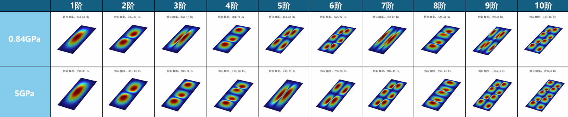
The image compares the first ten modes of two plate models, labelled 0.84 GPa and 5 GPa. GPa is a pressure unit commonly used for elastic modulus. It describes resistance to a specified deformation in the selected material model. It is neither a loudness unit nor a tone-quality score. Mode order gives a position in that model’s frequency ranking, not a listening grade.
Read the colour legend
Check the colour legend too. Many simulations display normalized displacement magnitude: red means relatively large and blue relatively small. Such a plot need not show the sign of motion. It does not show temperature unless the legend says so. Our earlier conceptual diagram deliberately used red and blue for opposite directions. Similar-looking colour maps can therefore represent different quantities.
A mode can exist without appearing clearly in one measurement
Mode shape and excitation point
Adjustable teaching modelTry it · Choose the transverse dipole and move the strike to 0.50. Then increase only the equivalent mass and observe the lower natural frequency.
5. The air does more than add a bass peak
Video reference: approximately 03:04–04:20
A bottle opening as an introduction to Helmholtz resonance
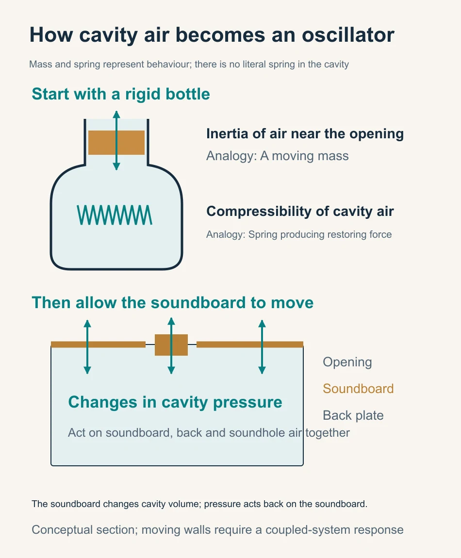
Blowing across a bottle opening excites air with inertia near its mouth. Compressing the air inside produces a restoring pressure. Represent the first behaviour by a mass and the second by a spring. This gives an intuitive model of Helmholtz resonance. It describes two ways of storing energy. There is no literal spring inside the air.
The approximation requires a wavelength much larger than the cavity, so the internal pressure can be treated as nearly uniform at each instant. With rigid walls, the opening area, cavity volume and effective acoustic length of the opening determine the characteristic frequency. Effective length includes the inertia of nearby air on both sides of the opening. It is not simply the soundboard thickness, and the correction changes with the opening’s shape and surroundings.
Moving walls change the whole system
Unlike a rigid bottle, a guitar has a moving soundboard and back. Inward soundboard motion changes cavity volume and pressure. That pressure drives air near the soundhole and exerts forces back on both plates. This is coupling. The wood does not finish vibrating before the air processes its output: each part influences the other’s motion as the vibration unfolds.
In the script’s two-degree-of-freedom teaching example, the unloaded soundboard has a reference frequency of 150 Hz. The rigid-wall air resonance is approximately 130 Hz. Using the mass, area, cavity volume and circular-opening parameters in the figure, and neglecting damping, the coupled system has frequencies near 97 and 201 Hz. Both modes involve soundboard and air motion. Neither belongs exclusively to the wood or exclusively to the air.
This is why an isolated “wood EQ” and an isolated “air EQ” cannot simply be connected in series. Coupling changes the loads and boundaries experienced by both. First solve the coupled system, then define its external input and output and the corresponding frequency response. At higher frequencies, more complex cavity modes also appear, beyond the scope of a single air spring.
Two coupled top–air modes
Adjustable teaching modelTry it · Change only the soundhole diameter and watch both modal frequencies and the top response. Compare the directions of x and y in the two modes.
Distinguish coupling, dissipation and overlapping peaks
Coupling can transfer energy from one part to another and back again. Without external forces or losses, the model’s total energy remains conserved. A smaller response at one point may simply mean that motion or energy has shifted elsewhere. It does not by itself prove conversion to heat or radiation into the far field.
The video illustrates coupling through the shared motion of components with nearby frequencies. A further distinction is needed: two nearby response peaks may broaden through damping until they appear as one unresolved hump. That single hump does not prove that the vibrations have synchronized or locked to one frequency. Changing a soundhole opening also changes boundary conditions, added air inertia and flow losses. One such adjustment cannot isolate every air parameter.
With these conditions clear, the air’s role is more precise: it changes the coupled system’s frequencies, mode shapes, phase relationships and energy distribution. For further background, see UNSW’s explanation of Helmholtz resonance and flexible guitar bodies. To understand why the sound eventually fades, we must also consider dissipation and sound radiation.
6. As a note decays, its timbre continues to change
Video reference: approximately 04:21–05:25
First define the system whose energy you are tracking
Energy transferred into the body has left the string, but it may remain stored in the combined string–body system and can return to the string. Likewise, sound energy radiated into the surrounding air is an output from the structure and an input to the acoustic field. Before calling something a loss, specify the system boundary used for the energy account.
Structural vibration decays through material losses, joint losses, thermoviscous losses in air and sound radiation, among other mechanisms. The dissipative processes irreversibly convert mechanical energy into heat. Radiation carries energy into a propagating sound field. All can contribute to effective structural damping, but they do not all mean that energy becomes heat inside the wood.
Local energy exchange through coupling differs from irreversible loss. Smaller displacement at one point may accompany greater motion elsewhere, in another direction or another mode. Lower pressure at one microphone may result from cancellation. To trace energy, consider the system boundary, motion and power together.
Why a narrow peak is related to a long decay
Consider a lightly damped, approximately isolated mode, with other conditions unchanged. Lower losses generally produce a narrower resonance peak and a slower free decay. Greater losses broaden the peak and shorten the decay. These are frequency-domain and time-domain views of the same dynamics, rather than independent sound effects.
Q ≈ fₙ / Δf
Q is a dimensionless measure of resonance sharpness, fₙ the modal natural frequency and Δf the half-power bandwidth. This approximation assumes light damping and sufficiently separated modes. Q is not a rating of instrument quality.
As a separate example, a 220 Hz mode takes about 0.60 seconds to lose 60 dB of amplitude at Q=60, or 0.20 seconds at Q=20. These times describe that mode in free decay. They are not the sustain of a whole string note or a room reverberation time. Even at the same Q, different frequencies give different decay times in seconds.
When estimating damping, distinguish amplitude, energy and their decibel representations. For a given form of motion, energy scales approximately with amplitude squared. Using the appropriate decibel definition makes these descriptions consistent. A software peak-hold fall rate, or the width of a recorded harmonic’s FFT peak, is not automatically a measurement of body-mode damping.
Timbre is not a frozen spectrum
A note contains components that may decay at different rates. For example, strong high-frequency components at the attack may weaken relative to the rest as the note develops. The video illustrates this as high frequencies fading before low ones. That sequence must be checked for the particular guitar, note and observation point; it is not a universal law.
A timbre that evolves over time does not necessarily imply changing system parameters. A linear system with fixed parameters and several decaying components can already produce changing spectral proportions after a pluck. Impulse response and convolution describe this memory of earlier excitation.
The video suggests that an instrument with no damping could vibrate indefinitely but remain inaudible. The key point is that sustained outward radiation removes stored structural energy when no external source replenishes it. Radiation is itself a damping mechanism. Thus a completely undamped system cannot also radiate sound continuously without an external energy supply. This does not make greater material loss inherently desirable, nor establish a universal rule that louder guitars must sustain for less time.
Describing decay with quantities we can compare
Damping in frequency and time
Adjustable teaching modelTry it · Hold frequency fixed and raise Q. Then hold Q fixed and raise frequency. Equal Q does not mean equal decay time in seconds.
Noise floor and beating
The noise floor also limits decay measurements in recordings. Once a component falls into background noise, its further decay becomes difficult to estimate. Disappearing from a display does not mean that mechanical motion becomes exactly zero at that moment. Two nearby frequencies can also produce beating, with alternating reinforcement and cancellation. A dip in the envelope need not indicate a sudden large energy loss; the contributions may reinforce again later.
Before assigning a decay time, specify the time interval, frequency band and amplitude quantity being analysed. State whether sustained driving has ended and whether the signal-to-noise ratio is adequate. Cross-checking time, frequency and phase information is more reliable than judging a structure from an attractive decay curve alone.
7. Convolution in guitar acoustics: connecting input and response
Video reference: approximately 05:30–06:03
Build a continuous input from small contributions
Imagine dividing the dynamic force at the bridge into many small contributions arriving at successive times. Each produces a response in the defined system. Within a linear approximation, shift each response to its starting time, scale it by the input strength, and add all contributions present at each instant. This operation is convolution.
The response following a very short force impulse provides an intuitive introduction to impulse response. It includes the later phase relationships, delays and decay, not just the initial movement. Earlier pushes can therefore influence the present, making the body an equalizer with memory. Convolution adds no extra physical stage to the energy flow; it is a way to calculate how input and system memory combine.
Output = Input ∗ Impulse Response
The asterisk denotes convolution, rather than ordinary multiplication of two values at the same instant. Define input, output and response consistently—for example, bridge force in a specified direction and sound pressure at a fixed receiving point.
Build a convolution term by term
Adjustable teaching modelTry it · Select alternating signs and add terms one at a time. See responses reinforce at some times and cancel at others.
A useful black box still needs clearly defined interfaces
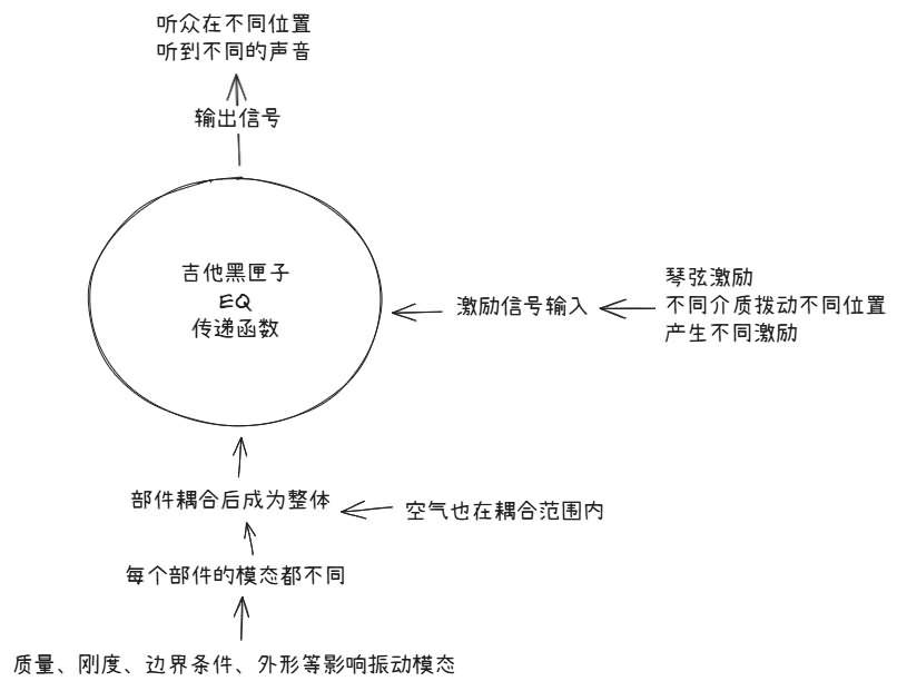
The sketch organizes three questions: where the input comes from, how the complete guitar responds, and where the output is observed. It does not mean that any string waveform can be fed unchanged into a box labelled body EQ. If the input is bridge force, the response units and system boundary must match that definition. If the starting point is the string shape before release, a complete dynamical description of the initial state is also needed.
Mass, stiffness, shape and boundary conditions are system parameters, with a different role from a driving signal that varies over time. Moving the plucking point mainly changes the current excitation. Changing supports, structure or air loading may change the system itself. This distinction tells us whether we are comparing different inputs to one system or different systems under a common input.
In the frequency domain, retain both magnitude and phase
In the frequency domain, convolution becomes multiplication of the input spectrum by the complex frequency response at each frequency. Magnitudes multiply and phases add. Relative strengths and the time alignment of components can therefore change. A magnitude curve alone cannot establish an exact reconstruction of the attack and decay.
Modes, coupling, damping and any included propagation conditions already contribute to the defined response. Convolving the input with it therefore includes the corresponding decay. Multiplying by an extra damping envelope without justification may count the same loss twice. Similarly, air effects included in a coupled response must not be added again as a separate EQ.
A compact formula requires consistent system boundaries
If the input is the actual bridge force measured synchronously, the response should describe the receiving body–air subsystem and the chosen output location. Do not count again the string feedback already represented in that internal bridge force. To predict the complete system from release instead, specify the full initial state of string, structure and air. Bridge force can then emerge from the coupled solution, rather than being added as an independent external input.
Before using the compact convolution formula, account for energy already stored at release through the input history or initial conditions. External recording and playback stages can be connected through their responses when interfaces, units and assumptions match. Internally interacting components, however, cannot be treated indiscriminately as a chain of one-way boxes.
The model assumes approximate linearity and stable conditions during the test. Does doubling the input double the response? Can separate responses be added? These questions help explain linearity. Fret buzz, clipping, large-amplitude contact and processing such as automatic gain control or compression can violate the assumptions. Useful models also need clear limits.
8. From body to room: one guitar, different sound at different positions
Corresponding video approximately 06:04–06:32
Disturbance and energy travel outward
Motion of the soundboard, back and air near the soundhole creates alternating compression and rarefaction in the surrounding air. In a small-amplitude sound wave, air particles mainly move back and forth near equilibrium. The pressure disturbance and energy propagate outward; a parcel of air does not fly all the way from the guitar into the ear. Local air motion and outward wave propagation are different things.
Pressure contributions from different parts of the body combine at a receiving point with their propagation distances and phases. They can reinforce in some directions and partly cancel in others. As frequency changes, so does the wavelength relative to the body’s size. A guitar’s radiation pattern therefore varies with frequency.
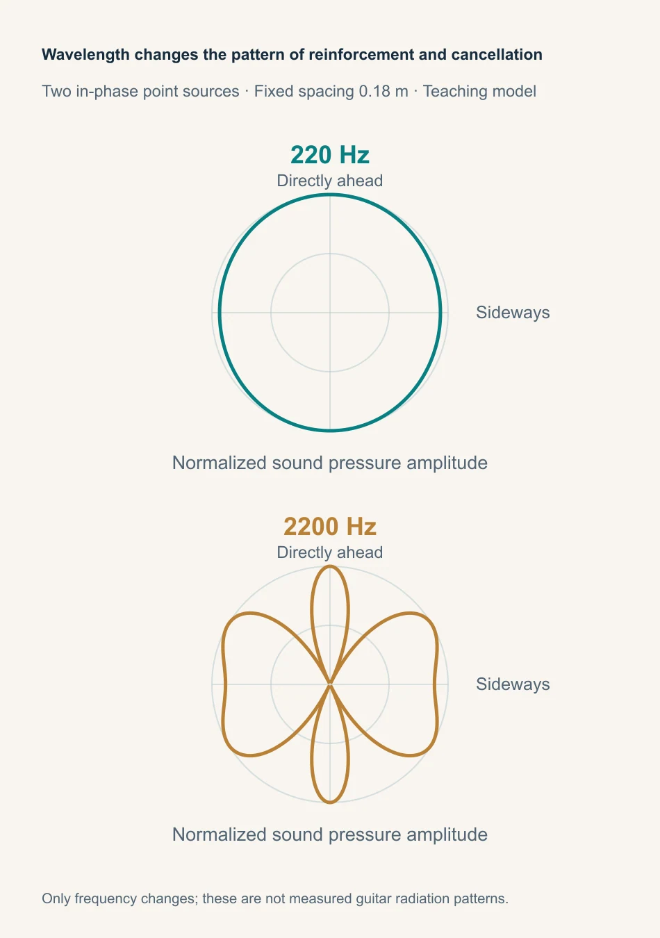
One microphone position cannot represent the entire sound field
The constant-pressure surfaces in the video make an invisible spatial pressure distribution visible. Moving your ears or microphone can change the spectral balance even when the instrument and playing stay the same. Large motion in one soundboard region does not guarantee efficient radiation in every direction. The phase relationships between regions matter too.
Pressure at one point is not the total acoustic power radiated in all directions. Cancellation at that point does not mean a reduction everywhere or the disappearance of energy. Comparisons of projection or radiation efficiency need stated distances, directions, frequency bands and measurement methods. One microphone response cannot represent the whole surrounding space.
Room reflections add further contributions. Direct and reflected sound travel different paths and combine at the microphone with different phases. Some frequencies strengthen and others weaken, producing a hollow, thin, full or otherwise coloured sound. Changing microphone distance and angle changes direct-sound sampling, reflected contributions and phase relationships. It does not establish a structural change in the guitar.
9. From pressure at the ear to the timbre we recognize
Corresponding video approximately 06:33–06:55
The cochlea’s frequency selectivity offers a useful starting point
Sound passes through the pinna and ear canal, drives the eardrum and middle-ear bones, and then sets cochlear fluid and structures in motion. Different regions of the basilar membrane are most sensitive to different frequencies: higher frequencies near the base and lower frequencies toward the apex. Hair cells convert mechanical stimulation into electrical signals, which travel along the auditory pathway to the brain.
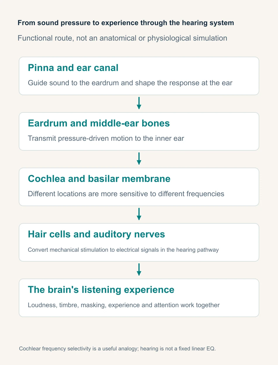
Longitudinal waves and hearing
Adjustable teaching modelTry it · Follow the red particle, then the travelling compression band. Raise the frequency and watch the wavelength shrink.
The video’s comparison of the cochlea to a spectrum analyser is an introductory analogy. Cochlear motion does have a frequency-dependent spatial pattern, but hearing involves much more than displaying a spectrum. The cochlea includes active, nonlinear processes; neural coding and brain recognition are also more complex than a fixed EQ. For an introduction to the hearing pathway, see NIDCD’s explanation.
Physical differences and listening preferences are connected, distinct questions
Perception also depends on loudness, masking, changes over time, playback equipment, attention and listening experience. A component visible in a spectrum is not necessarily easy to hear in a musical context. Physically different sounds may produce differences in perception that vary in salience. People’s outer ears, ear canals and hearing conditions differ, while their preferences also reflect experience.
Objective measurement remains valuable: it identifies which physical quantity changed and by how much. Controlled listening asks whether people can hear that change under specified conditions and whether they prefer it. Connecting these forms of evidence gives a clearer explanation than an impressive number or a description such as sounds more refined on its own.
10. From sounds different to an explanation we can test
The video introduces measurement around 02:58 and returns to the complete causal chain around 07:00.
Define the question before choosing the measurement
A recording can show which components reach a microphone during a particular pluck. To study how the bridge or soundboard moves under a given force, measure input and structural response. To identify a complete-system mode, use phase relationships across multiple measurement points and a suitable identification method. Different questions call for different instruments and evidence.
A spectrum analyser or software can reveal the frequency content of a chosen signal. Peaks in a playing recording, however, depend on plucking harmonics, the body, space, microphone and analysis window. Without a known input and defined input–output pair, that spectrum is not automatically an inventory of body modes. Calling a peak the soundboard’s natural frequency skips a claim that still needs evidence.
Normalize the laser response by hammer input
Adjustable teaching modelTry it · Double the strike force: velocity changes, but mobility does not. Then select a position near a node. The second peak weakens without the mode disappearing.
What a laboratory photograph tells us about the method
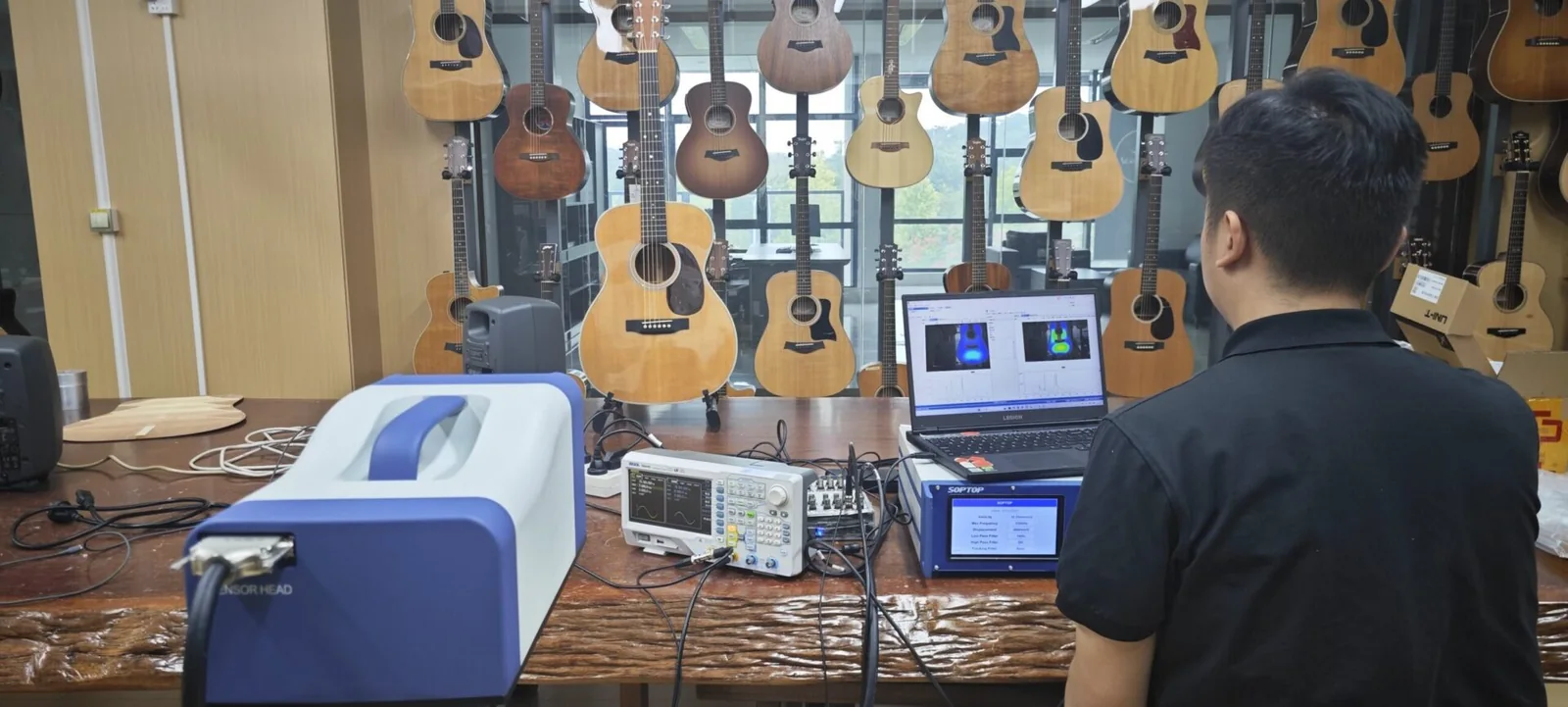
The laser, oscilloscope and computer in the photograph offer a practical way to observe structural motion. Laser vibrometry measures velocity along the beam without attaching a sensor to the point. Reflectivity, geometry and beam direction still affect the result. A coloured body plot on a screen cannot, by itself, identify a particular mode.
Combining an impact hammer and laser vibrometry
An instrumented impact hammer applies a short force and records the actual input. A laser vibrometer measures surface velocity in the selected beam direction. It does not automatically recover all three components of motion. Synchronous input and output support a force-to-velocity response estimate over a valid frequency band. A fixed microphone instead supports a force-to-pressure response at its location.
Simply dividing two arbitrary spectra does not guarantee a reliable response estimate. The hammer tip and impact technique determine the useful excitation band, while a double impact adds unwanted input. Windows, noise, coherence and repeated averaging also affect the estimate. Coherence helps assess the relationship between signals, but a high value alone does not validate the system boundary, linearity assumption or every measurement setting.
Keep a common amplitude and phase reference during scanning. Repeat measurements under consistent boundary conditions. Multi-point complex responses can then support modal identification with a suitable model. A scan under continuous single-frequency excitation initially shows an operating forced response. Identifying it as an individual mode requires further evidence.
From an impact to a reliable response and mode shape
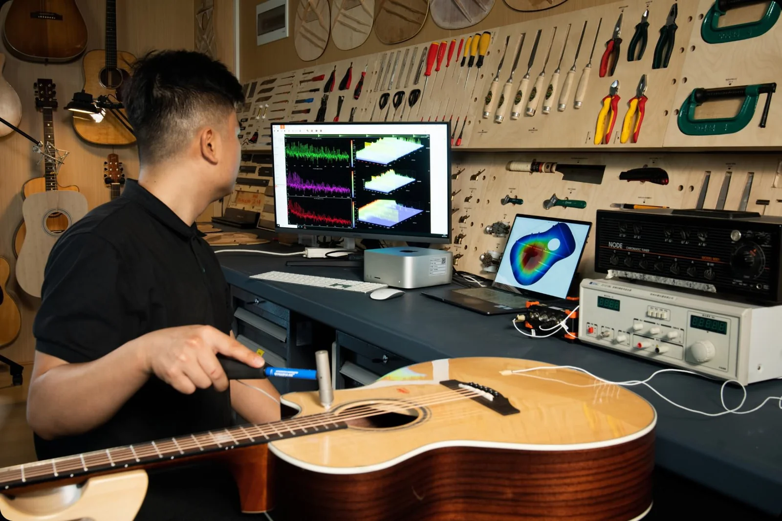
The hammer test turns a brief contact into a measured external input. Each impact need not have identical strength. It must remain within the useful linear range, and the actual force must be recorded. Then each output can be related to its own input. Merely comparing peak heights misses that reference. Fix or label impact locations and directions to avoid confusing input changes with structural changes.
Check measurement quality
Check the recordings before interpreting them. Look for clipping, double impacts, synchronization errors and insufficient input energy in the analysis band. Repeats help assess stability, but averaging cannot remove systematic error. An attached sensor also adds mass and mounting effects. Non-contact vibrometry avoids that attachment, while still requiring checks of beam direction and signal quality.
Conditions to document for a meaningful comparison
- Instrument and boundary conditions: String type and age, tuning, temperature, humidity, supports or playing posture, and whether strings are free or damped. Free and damped strings define different systems; do not treat their responses as one unchanged frequency response.
- Input and output: Plucking or impact location, direction and input-control method; vibration-sensor or microphone position, direction and distance; plot axes, units and normalization method.
- Repeat measurements and data processing: Number of valid repeats, criteria for rejecting data, sampling and analysis windows, noise and useful frequency band. Retain the original recordings before loudness matching.
What recording comparisons can still tell us
An online recording captures the complete chain: playing, strings, body, radiation direction, room, microphone, processing, playback and listener. It usually cannot uniquely reveal every stage’s properties. Different causes may produce similar spectral changes. A brighter recording alone therefore does not prove that a wood, brace design or structural parameter is better.
Controlled recordings can still support useful relative comparisons. Fix the recording chain and positions, alternate between guitars, repeat performances and document the conditions. For timbre comparisons, make separate listening copies with suitable loudness matching. This reduces a preference driven merely by greater level. Blind listening can reduce expectations from names and labels. Performance repeatability remains a limitation.
Loudness-matched listening copies do not establish which guitar produces greater actual pressure or radiates more efficiently under equal input. That question requires original, calibrated data and a defined excitation. Measurements should not end in one overall tone score either. Frequency response, decay, radiation, playability and preference describe different things and need interpretation around a clear question.
Separate the recording-chain variables
Adjustable teaching modelTry it · Set reflection to zero and change only the angle. Fix the angle and add reflection. Can these differences still be attributed solely to the guitar?
11. Putting guitar acoustics into a practical comparison
Comparison 1: change only the plucking position
Keep the same string, pitch, playing posture and microphone position. Alternate several times between plucks near the bridge and closer to the midpoint. Keep contact and release actions as consistent as possible, and compare attack, main tone and decay separately. You can place the recorded spectra beside the earlier interactive demonstration. The model predicts initial displacement-harmonic proportions; recordings also include body response, radiation and the recording chain. Their spectral lines should not be expected to coincide exactly.
Where possible, control the displacement before release and record the plucking position. Remember that equal displacement does not ensure equal input energy. This comparison asks how the recorded sound changes when the input to one guitar changes. It cannot establish one plucking position as the instrument’s unique, fixed timbre.
Comparison 2: keep the input reference and change the observation point
With synchronously measured impact-force input, keep the support and impact location and direction fixed while observing several structural or microphone positions. Identify features that persist and peaks or valleys that depend strongly on position. Use mode shapes and direction to investigate the cause. Keep a common reference scale: normalizing every curve to its own maximum hides some absolute differences and retains only within-curve proportions.
Ordinary recordings can also compare microphone positions while the player stays in place, but variations between performances limit the result. They cannot fully replace synchronous response measurements. Store tests with changed room, direction or distance separately from repeats under unchanged conditions, so those differences are not all attributed to guitar structure.
Comparison 3: record measured changes separately from preference
Before labelling a sound better or worse, describe its attack, the prominence of particular bands and the changing balance during decay. Check whether the data support those descriptions within the chosen analysis window. Measures such as spectral centroid can summarize frequency distribution, but specify the frequency band, time window and whether weighting uses magnitude or power. A higher value is not automatically a better tone.
Separate preference from discrimination
To compare preferences, retain the originals and prepare loudness-matched listening copies. Randomize or blind their order. Record two separate judgments: can listeners reliably distinguish them, and which do they prefer? For sound pressure or radiation efficiency at equal input, return to the appropriately calibrated, unmatched originals.
Connect every conclusion to its evidence
A useful record has three layers. First document conditions: string, pitch, support, excitation and microphone or sensor positions. Then record observations, such as a change in one band or modal response over a stated interval. Finally give the interpretation and note plausible alternatives. Later tests or parameter changes can then check whether that explanation still holds.
Listen again, and trace each difference to where it arises
After exploring guitar acoustics, pluck a string and follow the chain again. The fingers establish an initial state. The string applies force at the bridge and receives feedback. Structure and air respond through coupled modes, while components decay at different rates. Sound reinforces and cancels through space, then reaches playback and hearing. These processes overlap. The chapter sequence simply opens different views of one event.
We can enjoy a sound before we understand it. Science helps us explain that experience more clearly without replacing the experience itself.Return to the video and follow a single pluck again.
Sources and further reading
This article follows the Bilibili video The Physics of the Acoustic Guitar—Cosmic Afterglow. The detailed Before You Hear script supplies additional theory, measurement methods and limitations. Time references correspond to the approximately 08:16 version. Concept illustrations, teaching calculations and existing measurement photographs have distinct roles. Read each figure with its own colour legend, scale and stated conditions. Photographs do not replace complete measurement records. Interactive diagrams illustrate only the models and assumptions described beside them.
- UNSW: Strings, Standing Waves and Harmonics
- Helmholtz resonance and guitar corrections — UNSW
- UNSW: Guitar-acoustics measurements and sound radiation
- NIDCD: How we hear sounds
- ESA: Acoustic oscillations and structure formation in the early universe
- Kepma: Fundamentals of Guitar Modal Concepts
- NI: Understanding FFTs and Window Functions
- Polytec: Basic principles of laser Doppler vibrometry